

On tasks where the complexity needed to answer varies it makes intuitive sense that model complexity should vary accordingly. The ability to adaptively allocate more resources to difficult tasks is one that all humans possess and is evident in the increased requirements needed for complex mathematics compared to simple everyday tasks. This post introduces DACT [0], a new algorithm for achieving adaptive computation time that, unlike existing approaches, is fully differentiable. We put it to the test on Visual Reasoning datasets and find that our models learns to actively adapt their architectures according, balancing high accuracy with as-little-as-possible computation.
 |  | |
|---|---|---|
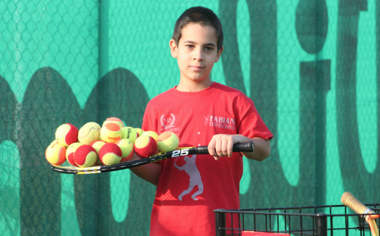
| How many balls is the kid holding? | How many birds is he holding? |
Visual Question Answering (VQA) [1] is a task where, for a given input image, question pair, we expect the model to return an answer. The difficulty of the task lies in the openness for both the question and image: because any image or plain-text question are valid expecting the model to output convincing answers can be seen as a more general Turing-test. These datasets pose challenging natural language questions about images whose solution requires the use of perceptual abilities, such as recognizing objects or attributes, identifying spatial relations, or implementing high-level capabilities like counting. For example, in the images above we see examples of two very similar (counting) questions for images from the Visual Genome dataset [2] that necessitate a broad understanding of the relation holding and a general purpose counting algorithm.
 |
|---|
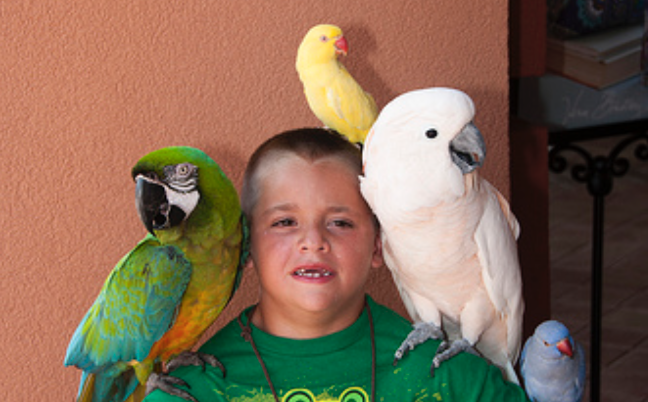
| Examples of questions in the CLEVR dataset that show a significant variation in the number of reasoning steps that are needed to answer them correctly. |
In open tasks such as this we find that instances entail diverse levels of complexity as both questions and images can be arbitrarily simple or difficult. Two examples from the CLEVR dataset [3] are shown above. Even in the very restricted subset of all possible images and questions included in this dataset (vocabulary of 28 words, generated images of the same objects) we find significant variation in complexity. Specifically, while the question of the first example involves just the identification of a specific attribute from a specific object, the second question requires the identification and comparative analysis of several attributes from several objects. We argue that dealing with this openness is paramount for more general intelligence and propose Adaptive Computation Time algorithms such as ACT [4] as possible solutions.
 |  | |
|---|---|---|
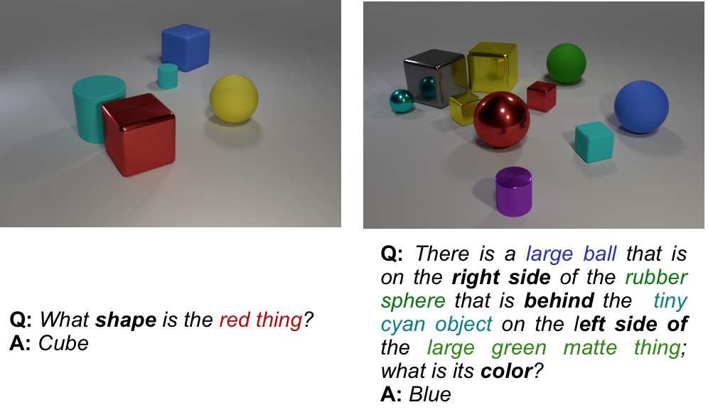
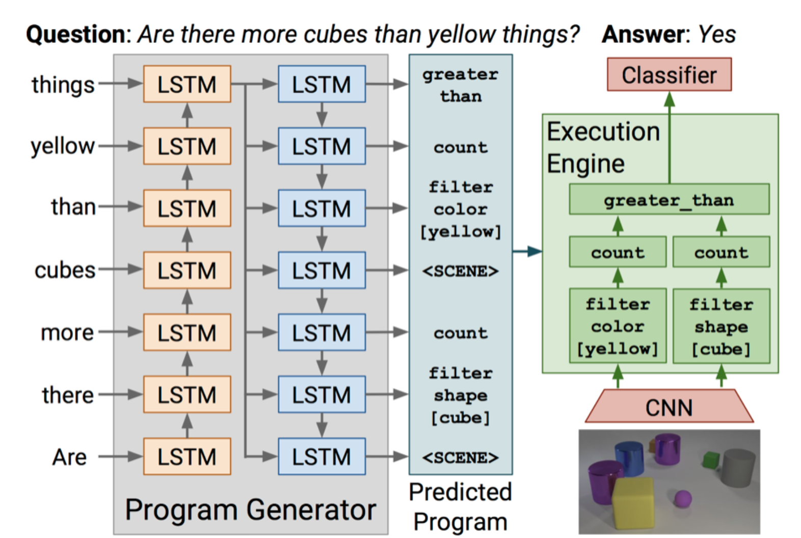
| Specialized Modules | General Purpose Module |
We consider modular networks those where modules are combined from a collection processing modules. Here we distinguish between two kinds:
Only the case of specialized modules is adaptive, but the generation of the sequences requires costly supervision or elaborate reinforcement learning training schemes.
The second case (general purpose modules) always executes the same module a fixed number of times, so no module selection training is needed. However, this approach is not adaptive as the processing pipeline is always the same. In our work, we build upon one of these networks by using DACT to adaptively select the horizon of the computational pipeline (instead of having it as a fixed hyper-parameter).
An algorithm for adaptive computation in neural networks already existed: ACT. I’ve already written a detailed explanation of how and why it works in a previous post, but the TLDR is that it works by forcing that the weights used to combine each step’s output into the final answer sum exactly one. To achieve this a non-differentiable piecewise function is used, namely: if the sum of the weights is more than one, then change the last weight so that the sum is exactly one. It has seen some success reducing computation in computer vision and natural language processing problems. However, we found that its theoretical shortcomings limited its usefulness for Visual Reasoning tasks (see Results), so we proposed a novel fully-differentiable algorithm.
 |
|---|
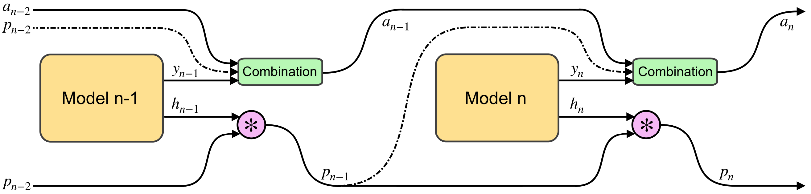
| The final answer Y is built up from the sub-answers from each module. The maximum contribution of any one of these steps is limited by all earlier ones, and any step can choose to limit contribution of subsequent ones. |
DACT was formulated as a differentiable alternative to ACT. In other words, it was designed to provide a means by which a model can halt computation without adding noise to the gradients.
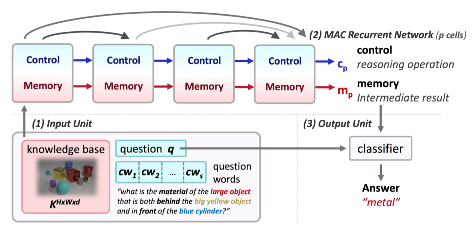
Our formulation can be applied to any model or ensemble that can be decomposed as a series of modules or submodels $m_n$, $n ∈ [1,…,N]$ that can be ordered by complexity. For example, recurrent networks are composed by iterative steps, CNNs by residual blocks, and ensembles by smaller models. We refer to the composition as our final model or ensemble $M$, and to its output as $Y$. This work focusses on its application to a recurrent visual reasoning architecture called MAC.
The core of the DACT algorithm is that any step can limit the total contribution of subsequent steps. To achieve this we use the sigmoidal halting values $h_n \in \left] 0, 1 \right[ $ to inductively define $p_n$ as:
\[p_n = \prod_{i=1}^{n}h_{i} = h_{n} p_{n-1}\]We observe that $p_n$ is monotonically decreasing for increasing values of $n$. Through their halting values each $n$th step can choose to either maintain the probability ($h_n \approx 1$) or reduce it ($h_n < 1$). The value of $p_n$ can be interpreted as the probability that a subsequent step might change the value of the final answer. Consequently, we define the initial value $p_0 = 1$.
The final answer $Y$ is built incrementally using the sub-answers of each step using accumulator variables $a_n$ for $n \in [1 \dots N]$ such that $Y = a_N$:
\[a_n = \begin{cases} \overrightarrow{0} & \text{if } n=0\\ y_n p_{n-1} + a_{n-1} \left( 1 - p_{n-1} \right) & \text{otherwise} \end{cases}\]It follows from this definition that $Y$ can always be rewritten as a weighted sum of intermediate outputs $y_n$. The relative relevance of each $y_n$ to the final output is thus constrained by $p_{n-1}$ which in turn is constrained by the $h_n$s of earlier steps.
We observe that this means that, for some step $n$ with low associated $p_n$, then $a_n \approx Y$.
During evaluation / test we want to identify the step where $a_n \approx Y$ to halt computation. How you choose to define $\approx$ in your code depends on you and the use-case. For this work we say that $a_n$ is similar enough to $Y$ once we are sure that the class with highest probability in $a_n$ is the same as in $Y$.
N = max_steps
for n in [1 ... N]:
    # run another step
    answer = run_module()

    if not answer_can_change():
        break
We say that the answer cannot change when the top class in $a_n$ will necessarily be the same as in $Y$ after all $d = N - n$ remaining steps. In particular, we are interested in checking if it’s possible that the probability associated to the runner up (second best) class $c^{ru}$ can surpass that of the top class ($c^*$).
def answer_can_change():
    d = N - n

    # get top and runner-up classes
    c_star = get_max_class(answer)
    c_ru = get_ru_class(answer)

    # check if answer cant change
    if min_p(c_star, d) >= max_p(c_ru, d):
        return False
    else:
        return True
The top answer is most likely to change if all $d$ remaining steps assign probability $0$ to $c^*$ and $1$ to $c^{ru}$. This scenario is the worst case from the perspective of the stability of the answer as it leads to the minimum value that the probability of class $c^*$ can take in $Y$; along with the maximum value for $c^{ru}$.
Then, after expanding the inductive definition of $a_n$ and replacing the worst-case probabilities we derive a lower bound for the probability of the class $c^*$ in $Y$:
\[\Pr(c^*, N) \geq \Pr(c^*, n)(1-p_n)^d\]And an upper bound to the probability of the runner-up class $c^{ru}$:
\[\Pr(c^{ru}, N) \leq \Pr(c^{ru}, n) + p_n d\]Therefore during inference we can safely cut computation once we identify a step $n$ such that we know for sure that the top classes in $a_n$ and $Y$ are the same. Mathematically, this means the halting condition is achieved when:
\[\Pr(c^*, n)(1-p_n)^d \geq \Pr(c^{ru}, n) + p_n d\](The math and some additional proofs are included in the paper.)
Finally, we add $\rho = \sum_{n=1}^{N} p_n$, a proxy of the total computation, to the loss function to encourage reduced computation:
\[\hat{L} (x, y) = L (x, y) + \tau \rho(x)\]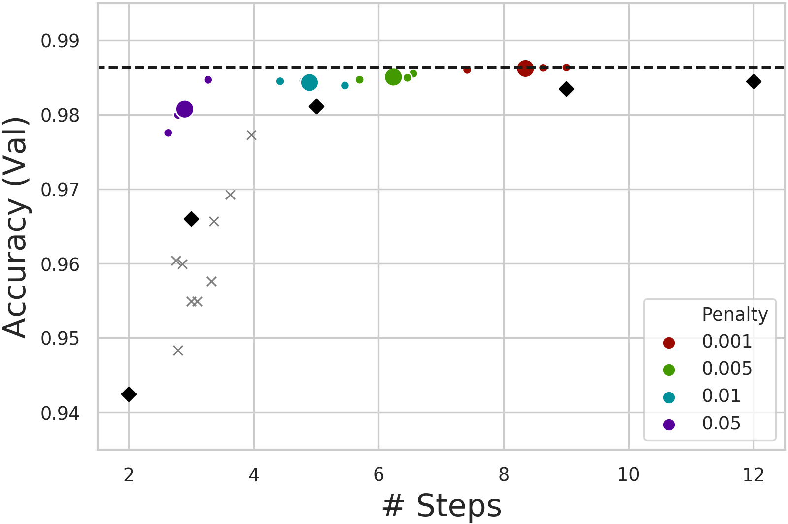 | 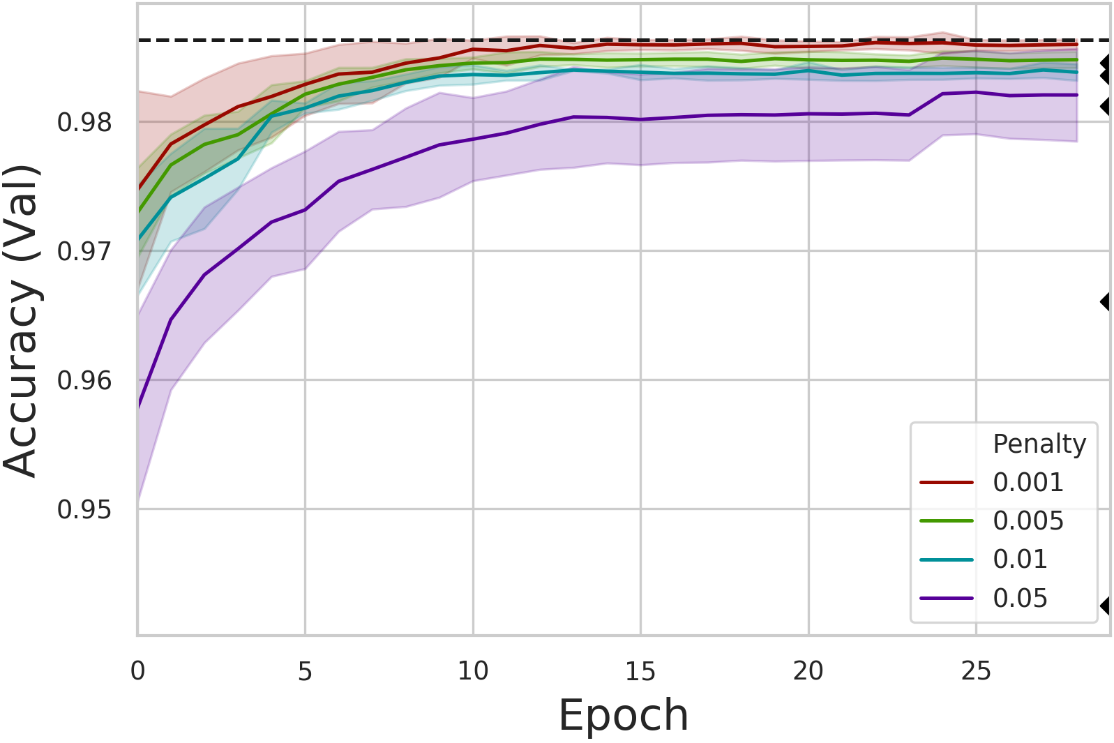 | |
|---|---|---|
| Scatterplot of computation (in steps) vs. precision. DACT-MACs shown in color; MACs as diamonds; ACT-MACs as crosses. | Learning curves for different regularization ( 𝜏 ponder cost) values show mean and variance of three runs. |
As the scatterplot above shows, DACT enabled MACs (in color) consistently outperform vanilla MACs (shown as diamonds) when both use comparable average numbers of steps. ACT on the other hand only performs as well or bellow as comparable MACs. Additionally, the figure shows that DACT responds predictably to changes in the penalty or ponder cost $\tau$ used (represented by the color), iterating fewer times when more penalty is used. This again contrasts with ACT which proved to be insensitive to the ponder cost. For instance, ACT without ponder cost ($\tau$ = 0.0) performs 3.2 steps on average and obtains an accuracy of 95.8%.
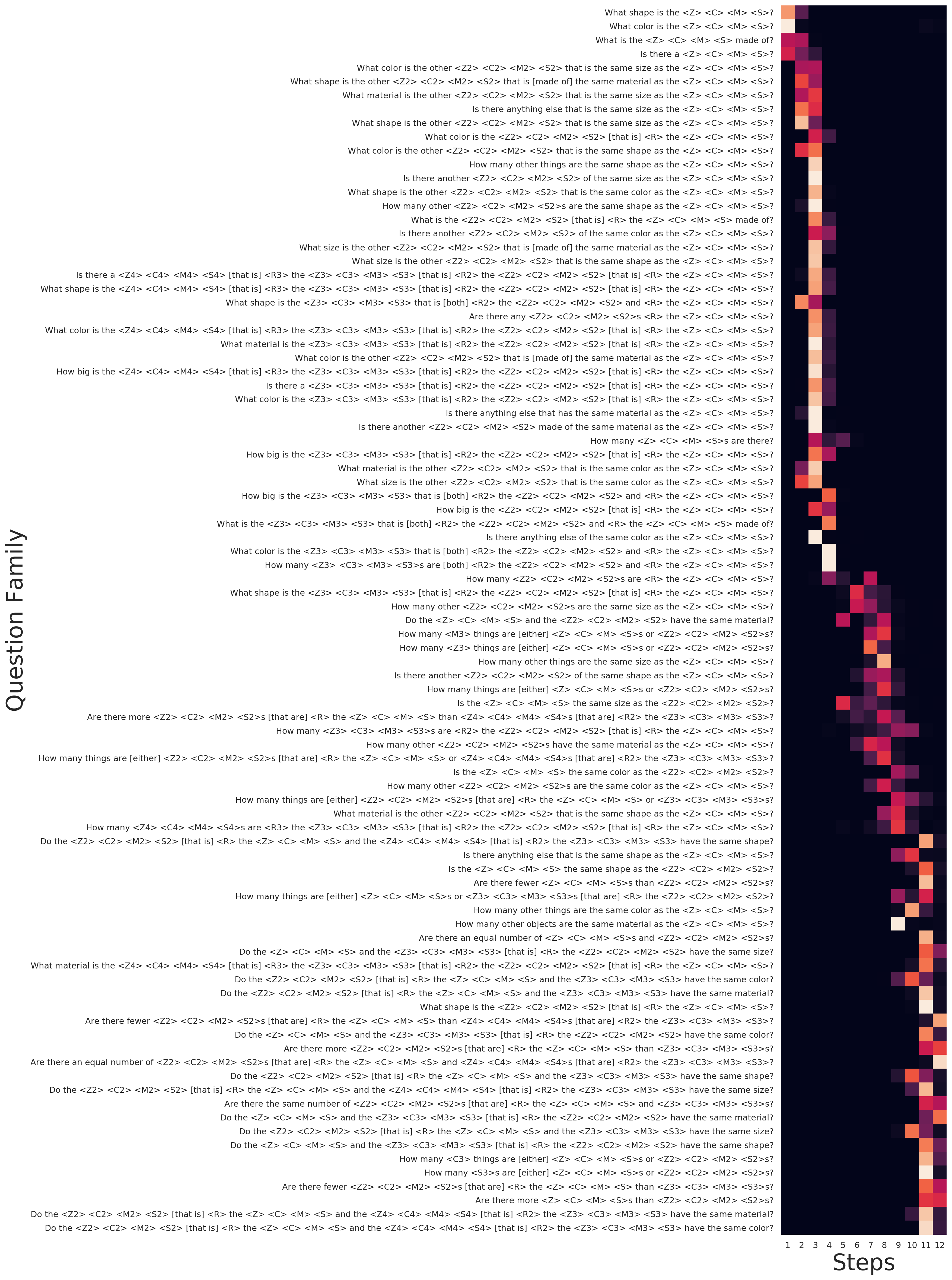
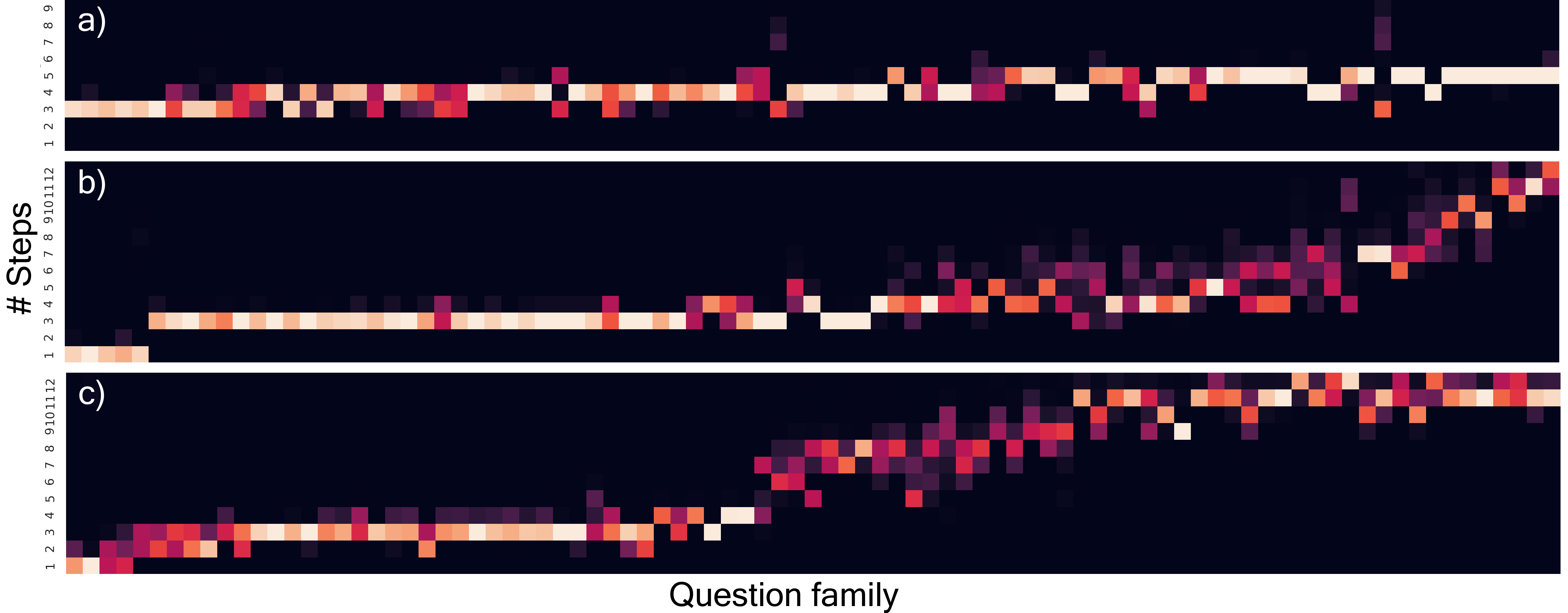 |
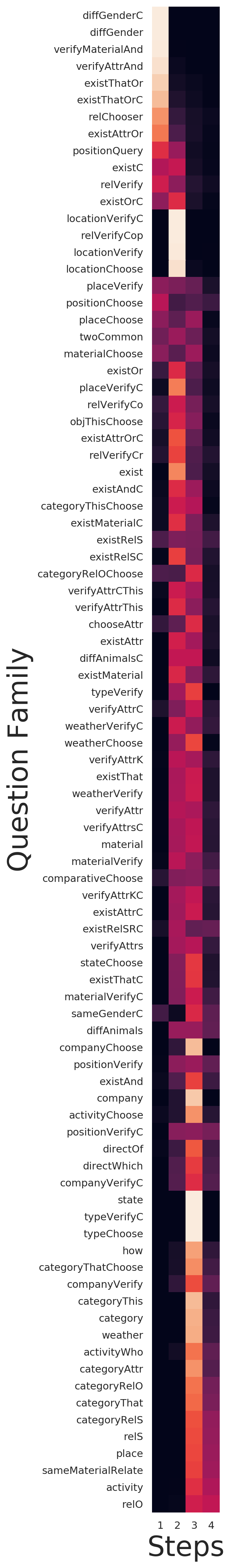
|---|
| How many steps are used by adaptive MACs for each question family in the CLEVR dataset. ACT-MACs in a); DACT-MACs shown in b) and c). |
The motivation behind using adaptive algorithms for this task is to use less computation for the more straightforward questions while still being able to use more computation for difficult ones. In the figure above a) shows the existing algorithm (ACT) failing to learn how to answer the most straightforward questions in less than three steps, or the hardest in more than five. The other two images show DACT using most of the available spectrum, showing that DACT enabled MACs are capable of actively allocating more computational resources to questions that need them. The second image b) shows a variant of DACT that averages approximately the same number of steps as a), while c) shows a DACT-MAC with lower ponder cost, which uses 50% more reasoning steps on average and thus achieves even better performance.
The figure shows questions clustered by family type which translates to groups that require similar step sequences to solve. The fact that DACT shows a remarkable correlation between computation and question family despite not including any type of supervision about these factors evinces the learning of meaningful patterns that correlate with question complexity. The full heatmap that shows an example for each question family can be found here.
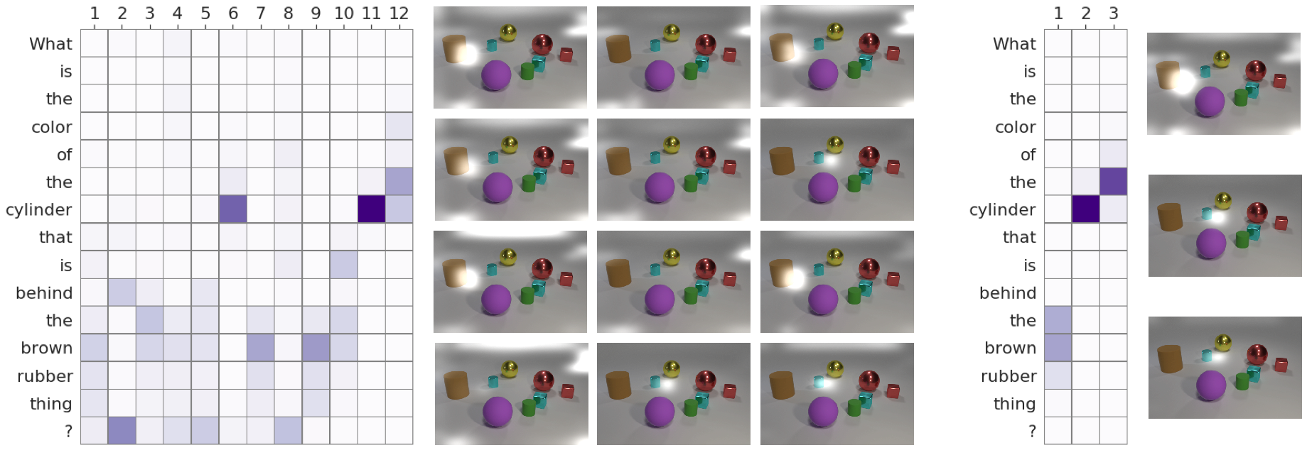 |
|---|
| Visual and linguistic attention maps for both regular MAC (left) and DACT-MAC (right). |
Besides the obvious and substantial reduction in the number of steps used to answer, our model also contributes to the overall interpretability of the inference. This is achieved by adding a proxy of the number of steps taken to the loss function, effectively coercing the model into only using fewer (and therefore more likely to be semantically strong) steps. This translates into more interpretable models. For instance, the question attentions above show that the last two steps are similar for both models, but that only one of the other ten steps used by MAC was necessary.
Additionally, the values of $p_n$ and the sub answers $a_n$ provide further insights.
Finally, in order to evaluate the generality of the suggested approach to real data, we evaluate the combined DACT-MAC architecture on the more diverse images and questions in the GQA dataset [7].
| Method | Ponder Cost | Steps | Accuracy |
|---|---|---|---|
| MAC+Gate | NA | 2 | 77.51 |
| MAC+Gate | NA | 3 | 77.52 |
| MAC+Gate | NA | 4 | 77.52 |
| MAC+Gate | NA | 5 | 77.36 |
| MAC+Gate | NA | 6 | 77.37 |
| ACT | 1e-2 | 1.99 | 77.17 |
| ACT | 1e-3 | 2.26 | 77.04 |
| ACT | 1e-4 | 2.31 | 77.21 |
| ACT | 0 | 2.15 | 77.20 |
| DACT | 5e-2 | 1.63 | 77.23 |
| DACT | 1e-2 | 2.77 | 77.26 |
| DACT | 5e-3 | 3.05 | 77.35 |
| DACT | 1e-3 | 3.69 | 77.31 |
We find that increasing computational steps doesn’t benefit the chosen architecture (MAC), and therefore adapting computation won’t increase performance. However, by adding DACT to a pre-trained 4-step MAC and then fine-tuning we find that it again outperforms the existing algorithm in terms of accuracy and responsiveness to ponder cost.
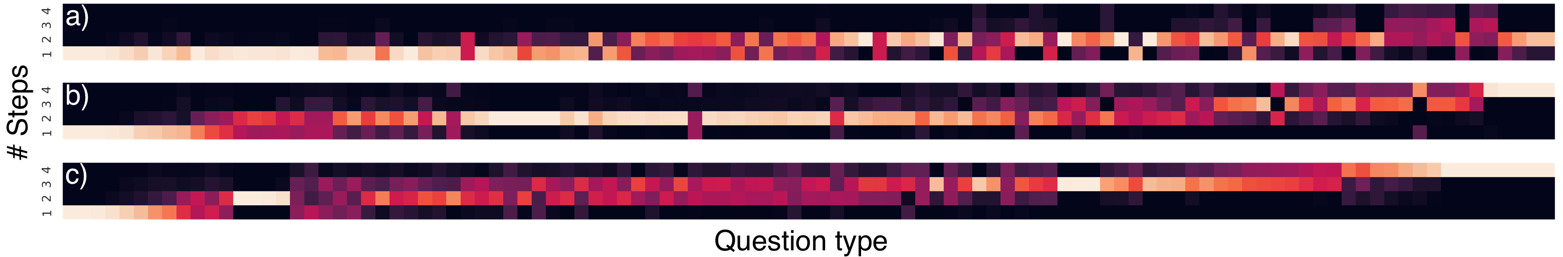 |
|---|
| How many steps are used by DACT-MACs for each question type in the GQA dataset. |
Additionally, we find that DACT-MACs adapt the 4-step algorithm reducing computation on some question types, and that the number of steps again correlate strongly with question types as can be seen in the heatmaps above. The same figures also show how the architecture adapts to changes in the ponder cost, as this penalty decreases DACT adaptively allocates more resources to more complex questions. The full heatmap that shows the question types can be found here.
A few lines for future work:
@article{Eyzaguirre2020DifferentiableAC,
  title={Differentiable Adaptive Computation Time for Visual Reasoning},
  author={Cristobal Eyzaguirre and A. Soto},
  journal={2020 IEEE/CVF Conference on Computer Vision and Pattern Recognition (CVPR)},
  year={2020},
  pages={12814-12822}
}