Adaptive Computation Time

Top-Down explanation of Graves’ 2015 paper “Adaptive Computation Time for Recurrent Neural Networks”

1. Motivation

Graves states “evidence that increased depth leads to more performant networks is by now inarguable, and recent results show that increased sequence length can be similarly beneficial”. The underlying principle seems to imply that putting your under-achieving model inside a recurrent network and have it iterate a fixed number of times (100 if you want) to observe better results. Of course, in practice the opposite seems to hold. The resulting model will be much more computationally intensive, will overfit to data easily and you probably wont even see gains in performance.

So what we need is a way to use these increased sequence lengths when more computation is required but at the same time prevent the network from overfitting. In other words, we want to increase the sequence length when needed, but limit complexity when it isn’t. How can we achieve this? By letting the network determine how many iterations it will run and including the number of iterations (or a proxy of this) in the loss function we should achieve a network that will iterate only when it helps to obtain a more accurate answer.

As we push towards a recurrent network that determines how many times it will iterate a new problem arises. How will the network determine its number of iterations? And how to make this differentiable? Having the network determine this limit a priori “would be equivalent to determining the Kolmogorov complexity of the data (and hence solving the halting problem)” (Graves, 2015). The solution proposed by Graves is to let the network halt when it is ready instead.

Pseudo code:

is_ready = False
answer = None
while True:
  # run model to update answer and check if ready
  answer, is_ready = run_model()
  if is_ready:
    break

2. Halting

For each iteration the network outputs an answer and a SIGMOIDAL halting value. The magnitude of the contribution of any iteration to the final answer $y_t$ is equal to the sub answer (the answer given by the iteration) multiplied by its probability of being relevant to the final answer $p_n$.

In order to limit computation we want all probabilities to be zero for $n > N$ (so that running for more iterations doesn’t change the answer).

A function $N$ is used to determine the first $n’$ for which the sum of all halting probabilities is greater than one minus a small epsilon. This is so that after one iteration the sigmoidal (and therefore never quite $1$) value of $h_n$ can be enough to halt if only one iteration is needed.

For each iteration $n$ before $n’$ the probability is equal to its halting value. Since the sum of all probabilities has to be equal to one (and we want to limit computation), for $n = N$ the probability $p_n$ will be equal to the remainder $R = 1 - \text{ the sum of all previous probabilities}$.

This way, for any $n > N$ the probability will be zero ($R = 1 - 1$), so we can get away with not computing them and the answer wont change, so:

Finally, we add a proxy of total computation $\rho = N + R$ to the loss to encourage reduced computation and backpropagate through this.

3. How it works

The main mechanism through which ACT operates is a non-differentiable piece-wise function. As such, the backpropagation of gradients through it is non-trivial.

Looking at the regularization term in the loss function $\rho$ we observe that no gradient can be propagated through $N$ and therefore adding $\rho$ to the loss is functionally equivalent to adding the remainder $R$. From it’s definition we observe that again no gradient can be propagated through the constant value $1$. Taken together this means that by adding $\rho$ to the loss function to minimize $text{loss} + \text{computation}$ we are actually minimizing $text{loss}$ while maximizing $\sum_{n=1}^{N-1}p_n$. By encouraging the network to maximize the halting probabilities of earlier steps we bias the network towards lower computation. This mechanism can be easily understood by considering that the $N$th step (the last answer-changing step) will be achieved earlier if, for instance, the first step greatly increases it’s halting probability.

4. Generalizing towards recurrent neural networks

In Graves’ work the process described above is repeated for each element $t$ in a sequence using an RNN. For each of these besides outputing $y_t$ (the $y$ for element $t$ of the sequence) a hidden state $s_t$ is computed:

Where $p_t^n \text{ is } p_n \text{ in timestep } t$.

And $N(t)$ is the first $n_t$ for which the sum of all $h_t^n$ is greater than one minus small epsilon.

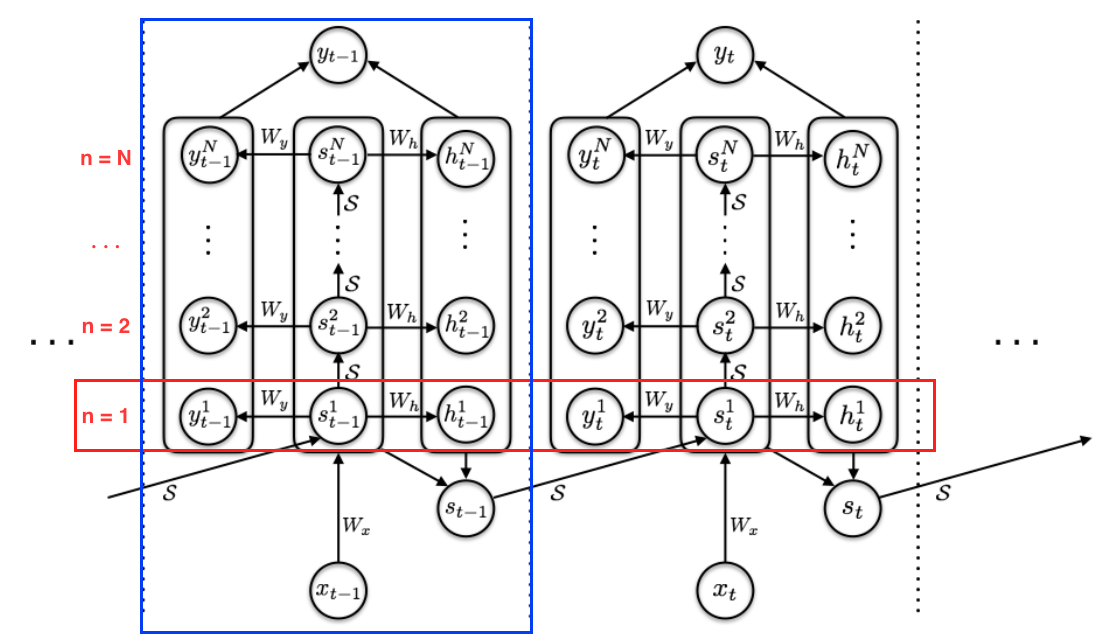
In blue is the process for one element of the sequence (as described in 2.). For each one of these elements $N(t)$ iterations are performed ($n = 1$ marked in red).

I haven’t talked about how to obtain any of the parameters mentioned (halting_values, sub_answers, sub_hidden_states) because it depends greatly on the implementation. A standard RNN (as shown in the image above) initializes its hidden state $s_t^1$ (when $n = 1$) to $S(s_{t-1}, x_t)$. In other words, for the first iteration of any element in the sequence the hidden state is a function $S$ applied to the COMPLETE hidden state at timestep $t - 1$ and the element of the sequence at index $t$. For any other iteration $s_t^n$ is $S(s_t^{n-1}, x_t)$.

Then both $y_t^n$ and $h_t^n$ are calculated by feeding the hidden state $s_t^n$ through feedforward layers $W_y$ and $W_h$ (with bias values) respectively. The output for the halting value $h_t^n$ is then squashed using a Sigmoid.